Graph Traversal Algorithms in Python: BFS and DFS Deep Dive with NetworkX
How to Read This Article
This article is written for readers with prior exposure to graph theory, algorithm analysis, and Python programming. It assumes familiarity with concepts such as graphs \( G = (V, E) \), adjacency representations, and asymptotic complexity.
The presentation intentionally blends formal mathematical reasoning with practical Python implementations using NetworkX. Mathematical notation and invariants are used where precision matters, while code examples illustrate how these ideas manifest in real systems.
You may read the article linearly, or jump directly to sections of interest. Advanced readers can skim implementation details and focus on traversal properties, structural implications, and performance discussions, returning to the code as needed.
I. Introduction
Graphs are one of the most fundamental data structures in mathematics and computer science, capturing relationships between entities via vertices (nodes) and edges (links). Formally, a graph is defined as:
\[G = (V, E)\]where \( V \) is a non-empty finite set of vertices, and \( E \) is a set of edges representing binary relations over \( V \). In an undirected graph, an edge \( e \in E \) is an unordered pair \( (u, v) \), while in a directed graph (or digraph), \( e = (u, v) \) is an ordered pair indicating a directed connection from \( u \) to \( v \).
Graphs are ubiquitous: they appear in transportation networks, social media, web indexing, biology, linguistics, compiler theory, and AI planning. Efficiently analyzing these structures often requires graph traversal algorithms, which systematically explore nodes and edges to extract structural and topological insights.
Why Traversal?
Traversal is not merely visiting nodes, it is the basis of solving a wide class of problems:
- Detecting cycles in dependency graphs
- Enumerating connected components in sparse networks .
- Constructing traversal trees for hierarchical representations
- Performing layered searches (e.g., BFS) for optimal reachability
- Classifying edges in directed acyclic graphs (DAGs)
Two canonical traversal algorithms are:
- Breadth-First Search (BFS): explores neighbors level by level using a queue (FIFO)
- Depth-First Search (DFS): explores as deep as possible before backtracking, typically using a stack (LIFO) or recursion
Both algorithms operate on the same input, the graph \(G = (V, E)\), but produce different traversal trees and expose different structural properties. From a theoretical standpoint, they offer insight into:
- Graph connectivity
- Path existence and reachability
- Layering and distance (BFS)
- Parent-child structure and edge classification (DFS)
Why NetworkX in Python?
While one could implement BFS and DFS from scratch using adjacency lists or matrices, the NetworkX
library provides:
- Clean abstractions over different graph types (e.g.,
Graph,DiGraph) - Support for both directed/undirected and weighted/unweighted graphs
- Efficient traversal utilities:
bfs_tree(),dfs_edges(), etc. - Integration with
matplotlibfor structural visualization
In this article, we will explore BFS and DFS both theoretically and practically. We'll analyze their computational complexity, traversal characteristics, and Python implementations using NetworkX. Our goal is not only to use these algorithms, but to understand their behavior deeply, mathematically, algorithmically, and visually.
II. Graph Representations
Before traversing a graph, we must choose how to represent it. The representation directly influences the algorithm's time and space complexity. Mathematically, a graph is defined as: \(G = (V, E)\) where \(V = \{v_1, v_2, ..., v_n\}\) is the vertex set (with cardinality \(n = |V|\)), and \(E ⊆ V × V\) is the edge set. In practice, we must encode \(E\) efficiently. Two classic representations are:
1. Adjacency Matrix
An \(n × n\) matrix \(A\) where:
A[i][j] =
    1   if there exists an edge from vertex i to vertex j
    0   otherwise
Formally: Let \(V = \{v_1, v_2, ..., v_n\}\), then the adjacency matrix \(A ∈ \{0,1\}^{n×n}\) is defined as:
\[A[i][j] = 1 ⟺ (v_i, v_j) ∈ E\]- Pros: Constant-time edge existence check: \(O(1)\)
- Cons: Space complexity: \(O(n²)\) regardless of sparsity
2. Adjacency List
A mapping from each vertex to a list (or set) of its adjacent vertices:
\[Adj(v) = \{u ∈ V | (v, u) ∈ E\}\]In Python, this is often implemented as a dictionary of lists or sets. For sparse graphs, this yields space complexity: \(O(n + m)\) where \(m = |E|\) This representation is optimal for traversal algorithms like BFS and DFS.
3. NetworkX Internal Representation
NetworkX abstracts graphs as Python objects, with adjacency list storage under the hood. For a simple graph:
import networkx as nx

G = nx.Graph()
G.add_edges_from([
    (1, 2), (1, 3), (2, 4), (3, 4)
])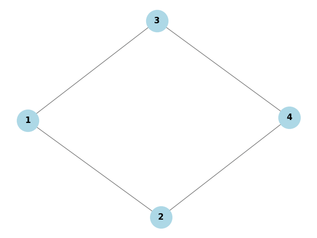
Internally, NetworkX stores:
G._adj = {
    1: {2: {}, 3: {}},
    2: {1: {}, 4: {}},
    3: {1: {}, 4: {}},
    4: {2: {}, 3: {}}
}
where each entry maps a node to its neighbors, with optional edge attribute dictionaries.
4. Directed and Weighted Graphs
NetworkX supports directed graphs via nx.DiGraph(), and edge weights can be stored as attributes:
DG = nx.DiGraph()
DG.add_edge('A', 'B', weight=3.7)
Mathematically, we interpret the edge set as a function:
\[E: V × V → ℝ^+\]where \(E(u, v)\) returns the edge weight between \(u\) and \(v\), if such an edge exists.
5. Sparse vs Dense Graphs
The density of a graph is defined as:
\[ D = \frac{2 \left| E \right|}{\left| V \right| \left( \left| V \right| - 1 \right)} \]For sparse graphs \(D ≪ 1\), adjacency lists are preferable. For dense graphs \(D → 1\), adjacency matrices allow faster edge queries, at the cost of space.
Summary
- Adjacency Matrix: Best for dense graphs, fast edge lookup, poor space efficiency
- Adjacency List: Best for traversal, scales well with sparse graphs
- NetworkX: Encapsulates both, uses adjacency list internally, and supports advanced graph operations with ease
In the next section, we will implement Breadth-First Search (BFS) and analyze its traversal properties and theoretical behavior.
III. Breadth-First Search (BFS)
Breadth-First Search (BFS) is a fundamental graph traversal algorithm that explores vertices in layers. It starts from a source vertex and visits all its immediate neighbors before proceeding to neighbors of neighbors, and so on.
1. Mathematical Model
Given a graph G = (V, E) and a source vertex s ∈ V, BFS computes the shortest path (in
terms of edge count) from s to every vertex reachable from s.
It constructs a level function:
L: V → ℕ ∪ \{∞\}
where L(v) is the number of edges on the shortest path from s to v. If
v is unreachable, L(v) = ∞.
The traversal forms a spanning tree (or forest in disconnected graphs), called the BFS tree,
rooted at s.
2. Algorithm Description
BFS uses a first-in-first-out (FIFO) queue to maintain the frontier of exploration.
Input: Graph G = (V, E), starting vertex s ∈ V
Output: Distances L(v) and BFS tree T

1. Initialize all L(v) ← ∞
2. Set L(s) ← 0
3. Create a queue Q and enqueue s
4. While Q ≠ ∅:
     u ← Q.dequeue()
     For each neighbor v of u:
         If L(v) = ∞:
             L(v) ← L(u) + 1
             Parent[v] ← u
             Enqueue v
Time complexity: O(|V| + |E|), assuming adjacency list representation.
3. BFS in Python using NetworkX
We begin with a simple undirected graph:
import networkx as nx

G = nx.Graph()
G.add_edges_from([
    ('A', 'B'), ('A', 'C'),
    ('B', 'D'), ('C', 'E'),
    ('D', 'F'), ('E', 'F')
])
NetworkX provides built-in BFS functions:
bfs_tree = nx.bfs_tree(G, source='A')
list(bfs_tree.edges())
# Output: [('A', 'B'), ('A', 'C'), ('B', 'D'), ('C', 'E'), ('D', 'F')]
This gives a BFS spanning tree rooted at 'A'.
Custom BFS Implementation
from collections import deque

def bfs_custom(graph, start):
    visited = set()
    level = {start: 0}
    parent = {start: None}
    queue = deque([start])

    while queue:
        u = queue.popleft()
        for v in graph.neighbors(u):
            if v not in visited:
                visited.add(v)
                level[v] = level[u] + 1
                parent[v] = u
                queue.append(v)
    return level, parent
This provides the layer (distance) of each node from the source, and the BFS tree via the parent
map.
4. Visualization of BFS Layers
We can visualize the BFS layers by mapping node colors to their distance from the source:
import matplotlib.pyplot as plt

level, _ = bfs_custom(G, 'A')
colors = [level.get(n, 0) for n in G.nodes]

pos = nx.spring_layout(G, seed=42)
nx.draw(G, pos, with_labels=True, node_color=colors, cmap=plt.cm.viridis)
plt.show()
The spring layout and colormap help illustrate how far each node is from the root, layer by layer.
5. Properties and Use Cases
- Shortest-path guarantee: For unweighted graphs, BFS finds the shortest path from
sto anyv. - Connected component exploration: BFS can enumerate all nodes reachable from a given vertex.
- Layered structure: Each frontier expands outward in discrete levels.
- Bipartite graph testing: Check if the graph can be 2-colored using BFS levels.
6. Theoretical Notes
-
The BFS tree is a subgraph
T ⊆ Gwhere for eachvreachable froms, the unique path inTis the shortest path inG. - On disconnected graphs, BFS produces a forest by restarting on unvisited vertices.
- For a DAG, BFS does not provide topological order, but it helps identify reachable vertices layer-wise.
In the next section, we’ll analyze Depth-First Search (DFS), including recursive structure, edge classification, and practical applications like cycle detection.
IV. Depth-First Search (DFS)
Depth-First Search (DFS) is a graph traversal algorithm that explores as far along each branch as possible before backtracking. Unlike BFS, which operates in levels, DFS uses depth-oriented exploration to uncover rich structural information.
1. Theoretical Framework
Given a graph G = (V, E), DFS constructs a spanning tree (or forest) by recursively visiting
unvisited neighbors. The traversal defines:
- Discovery time: The time a node is first visited
- Finish time: The time all descendants have been explored
Mathematically, DFS defines a parent function π: V → V ∪ {None} forming a rooted tree:
∀v ∈ V_reachable, π(v) is the vertex from which v was first discoveredDFS can be implemented recursively or iteratively via an explicit stack (LIFO). The time complexity is:
O(|V| + |E|)assuming adjacency list representation.
2. DFS Edge Classification
DFS traversals allow us to classify edges based on their relation to the DFS tree:
- Tree edge: First visit to an unvisited vertex
- Back edge: Edge to an ancestor (forms a cycle)
- Forward edge: Edge to a descendant (not tree edge)
- Cross edge: Edge between subtrees or unrelated vertices
Edge classification is meaningful in directed graphs. In undirected graphs, only tree and back edges appear.
3. DFS in Python using NetworkX
import networkx as nx

G = nx.DiGraph()
G.add_edges_from([
    ('A', 'B'), ('A', 'C'), ('B', 'D'), ('C', 'D'),
    ('D', 'E'), ('E', 'B')  # cycle: B → D → E → B
])

dfs_edges = list(nx.dfs_edges(G, source='A'))
print(dfs_edges)
# Output: [('A', 'B'), ('B', 'D'), ('D', 'E'), ('E', 'C')]
This shows the traversal path, forming a DFS tree starting at 'A'.
Tracking Discovery & Finish Time
time = 0
discovery = {}
finish = {}

def dfs_time(G, u, visited):
    global time
    visited.add(u)
    time += 1
    discovery[u] = time
    for v in G.neighbors(u):
        if v not in visited:
            dfs_time(G, v, visited)
    time += 1
    finish[u] = time

visited = set()
dfs_time(G, 'A', visited)
print(discovery)
print(finish)
This captures the discovery and finish times for each node, which can be used to classify edges.
4. Visualization of DFS Tree
DFS traversal builds a tree or forest depending on graph connectivity. We can highlight the tree edges:
import matplotlib.pyplot as plt

tree = nx.DiGraph()
tree.add_edges_from(dfs_edges)

pos = nx.spring_layout(G, seed=42)
nx.draw_networkx(G, pos, alpha=0.4)
nx.draw_networkx_edges(tree, pos, edge_color='red', width=2)
nx.draw_networkx_labels(G, pos)
plt.title("DFS Tree (Red)")
plt.show()
5. Applications of DFS
- Cycle detection: Presence of a back edge implies a cycle in a directed graph
- Topological sorting: DFS post-order yields valid order if DAG
- Connected components: Repeated DFS builds all connected subgraphs
- Bridge and articulation point detection: Using low-link values (Tarjan’s algorithm)
- Edge classification: Crucial in compiler optimizations and control-flow graphs
6. Theoretical Notes
- DFS defines a total order on vertices via finish time
- DFS tree is not unique: it depends on neighbor iteration order
- For DAGs, all back edges are absent → used for DAG validation
- DFS produces a depth-first forest if the graph is disconnected
In the next section, we will directly compare BFS and DFS across dimensions such as memory usage, traversal output, and algorithmic guarantees.
V. Comparative Analysis: BFS vs DFS
Although Breadth-First Search (BFS) and Depth-First Search (DFS) operate on the same graph
G = (V, E) and share identical asymptotic time complexity, they differ significantly
in traversal strategy, memory behavior, structural output, and suitability for specific problems.
1. Traversal Strategy
BFS explores the graph in concentric layers around a source vertex, while DFS explores a single path as deeply as possible before backtracking.
-
BFS: Maintains a frontier of nodes at distance
kbefore moving tok + 1 - DFS: Follows a depth-first recursion tree, delaying sibling exploration
Mathematically, BFS computes a shortest-path distance function
L: V → ℕ (edge count), whereas DFS does not preserve distance information.
2. Traversal Trees
Both algorithms produce spanning trees (or forests in disconnected graphs), but the structure of these trees differs:
- BFS Tree: Height-minimal with respect to the source
- DFS Tree: Depth-heavy, dependent on neighbor ordering
Let T_B be a BFS tree rooted at s. For every vertex v,
the unique path from s to v in T_B is a shortest path in G.
This property does not hold for DFS trees.
3. Memory Usage
Although both algorithms run in O(|V| + |E|) time, their memory usage differs:
- BFS: Requires memory proportional to the maximum width of the graph (queue size ≈ size of largest level)
- DFS: Requires memory proportional to the maximum depth of recursion (stack depth ≈ height of DFS tree)
In worst-case scenarios (e.g., complete graphs), BFS may consume significantly more memory than DFS.
4. Edge Information and Structural Insight
DFS provides richer structural information than BFS:
- DFS supports edge classification (tree, back, forward, cross)
- DFS discovery/finish times induce a partial ordering on vertices
- Back edges detected by DFS imply cycles in directed graphs
BFS does not produce finish times and does not distinguish edge types beyond tree/non-tree.
5. Applicability by Problem Class
| Problem Type | Preferred Algorithm | Reason |
|---|---|---|
| Shortest path (unweighted) | BFS | Layer-wise traversal guarantees minimal edge count |
| Cycle detection | DFS | Back-edge identification |
| Topological sorting | DFS | Post-order traversal yields valid ordering |
| Connected components | Either | Both enumerate reachable subgraphs |
| Bipartite testing | BFS | Level-based coloring |
6. Sensitivity to Graph Ordering
Both BFS and DFS are sensitive to the order in which neighbors are visited. NetworkX preserves insertion order, so traversal output may differ depending on graph construction.
This non-determinism is particularly important in DFS, where different traversal trees may expose different back edges or subtree structures.
7. Summary Comparison
- BFS: Optimal for distance-based exploration and layering
- DFS: Optimal for structural analysis and graph decomposition
- Both are linear-time algorithms with complementary strengths
In the next section, we will examine how BFS and DFS behave on directed and weighted graphs, and what guarantees are preserved or lost in these contexts.
VI. Traversal on Directed and Weighted Graphs
Thus far, our discussion of BFS and DFS has implicitly assumed undirected, unweighted graphs. In this section, we extend the analysis to directed and weighted graphs, and examine which theoretical guarantees remain valid and which do not.
1. Directed Graphs: Asymmetric Reachability
A directed graph (digraph) is defined as:
\[ G = (V, E), \quad \text{where } E \subseteq V \times V \]
An edge (u, v) represents a one-way relation from u to v.
Reachability is therefore asymmetric:
Both BFS and DFS operate without modification on directed graphs, but their traversal behavior changes fundamentally due to edge directionality.
2. BFS on Directed Graphs
BFS on a directed graph computes shortest paths (in terms of number of directed edges)
from a source vertex s to all vertices reachable from s.
The level function remains well-defined:
\[ L(v) = \min \{ \text{number of directed edges on any path from } s \text{ to } v \} \]However, BFS cannot infer reachability in the reverse direction unless corresponding edges exist.
import networkx as nx

DG = nx.DiGraph()
DG.add_edges_from([
    ('A', 'B'), ('B', 'C'), ('C', 'D')
])

list(nx.bfs_tree(DG, source='A').edges())
# Output: [('A', 'B'), ('B', 'C'), ('C', 'D')]
Starting BFS from 'D' would yield no edges, as no outgoing edges exist.
3. DFS on Directed Graphs
DFS on directed graphs is significantly more informative than BFS due to edge classification.
Using discovery time \(d(v)\) and finish time \(f(v)\), DFS classifies edges as:
- Tree edge:
(u, v)wherevis first discovered fromu - Back edge:
(u, v)wherevis an ancestor ofu - Forward edge:
(u, v)wherevis a descendant ofu - Cross edge: All other edges
A back edge exists if and only if the directed graph contains a cycle. This makes DFS the foundation for:
- Cycle detection
- DAG validation
- Topological sorting
- Strongly connected component algorithms
4. Traversal on Weighted Graphs
A weighted graph augments the edge set with a weight function:
\[ w : E \rightarrow \mathbb{R} \]BFS and DFS ignore edge weights entirely. Traversal decisions depend only on graph topology, not on cost.
Consequently:
- BFS does not compute shortest paths in weighted graphs
- DFS provides no distance guarantees of any kind
WG = nx.Graph()
WG.add_edge('A', 'B', weight=100)
WG.add_edge('A', 'C', weight=1)
WG.add_edge('C', 'B', weight=1)

list(nx.bfs_tree(WG, source='A').edges())
# BFS may explore A → B before A → C
Even though the path A → C → B has lower total weight, BFS is oblivious
to this fact.
5. Theoretical Implications
- BFS shortest-path guarantees apply only to unweighted graphs (or graphs with uniform weights)
- DFS remains useful for structural analysis regardless of weights
- Weighted shortest-path problems require fundamentally different algorithms (e.g., Dijkstra, Bellman–Ford)
6. Practical Guidance
- Use BFS for reachability and hop-count distance in directed graphs
- Use DFS for cycle detection, DAG analysis, and graph decomposition
- Do not rely on BFS or DFS for cost-based optimization problems
In the next section, we will formalize traversal trees and forests, and analyze how BFS and DFS induce different structural decompositions of the same graph.
VII. Traversal Trees and Forests
Both Breadth-First Search (BFS) and Depth-First Search (DFS) induce structured subgraphs during traversal. These structures are not arbitrary; they are formally defined spanning trees or spanning forests of the original graph.
Understanding these induced structures is essential, as many higher-level graph algorithms are defined in terms of traversal trees rather than the original graph.
1. Traversal Tree: Formal Definition
Let \( G = (V, E) \) be a graph and let \( s \in V \) be a chosen start vertex. A traversal algorithm defines a parent function:
\[ \pi : V \rightarrow V \cup \{\varnothing\} \]
such that:
- \( \pi(s) = \varnothing \)
- \( \pi(v) = u \) if and only if \( u \) is the vertex from which \( v \) was first discovered
The set of edges:
\[ E_T = \{ (\pi(v), v) \mid v \in V, \pi(v) \neq \varnothing \} \]
defines a tree \( T = (V_T, E_T) \), where \( V_T \subseteq V \). This is called the traversal tree.
2. BFS Trees
In BFS, the traversal tree is called a BFS tree. It has a defining optimality property:
\[ \forall v \in V_T,\quad d_T(s, v) = d_G(s, v) \]
where:
- \( d_G(s, v) \): shortest-path distance in \( G \) measured in number of edges
- \( d_T(s, v) \): path length in the BFS tree
This means the BFS tree preserves shortest paths from the source to every reachable vertex. Consequently, BFS trees are level-preserving.
Define the level function:
\[ L(v) = d_G(s, v) \]
Then for every tree edge \( (u, v) \in E_T \):
\[ L(v) = L(u) + 1 \]
3. DFS Trees
In DFS, the traversal tree reflects the recursive structure of exploration. DFS defines two timestamps for each vertex \( v \):
- \( d(v) \): discovery time
- \( f(v) \): finish time
These times satisfy:
\[ d(v) < f(v) \]
and induce a strict nesting property:
\[ [d(u), f(u)] \cap [d(v), f(v)] \neq \varnothing \;\Longrightarrow\; [d(u), f(u)] \subseteq [d(v), f(v)] \;\text{or}\; [d(v), f(v)] \subseteq [d(u), f(u)] \]
This interval nesting captures ancestor–descendant relationships in the DFS tree.
4. Traversal Forests
If the graph \( G \) is disconnected, BFS or DFS starting from a single vertex will only cover one connected component.
To traverse the entire graph, we repeat the traversal for each unvisited vertex. The result is a spanning forest:
\[ \mathcal{F} = \{ T_1, T_2, \dots, T_k \} \]
where each \( T_i \) is a traversal tree of a connected component of \( G \).
The parent function generalizes naturally:
\[ \pi : V \rightarrow V \cup \{\varnothing\}, \quad \pi(v) = \varnothing \text{ if } v \text{ is a root of some } T_i \]
5. Structural Consequences
- BFS forests preserve shortest-path distances within each component
- DFS forests encode hierarchical decomposition of the graph
- Edge classification (tree, back, forward, cross) is defined with respect to DFS trees
- Many graph algorithms operate purely on traversal trees rather than the full graph
6. NetworkX Extraction
NetworkX exposes traversal trees directly:
bfs_tree = nx.bfs_tree(G, source=s)
dfs_tree = nx.dfs_tree(G, source=s)
These trees are themselves graphs, enabling recursive analysis, visualization, and further algorithmic processing.
In the next section, we will examine real-world and research applications where traversal trees and forests play a central role.
VIII. Graph Traversal Applications in Research and Industry
Graph traversal algorithms are rarely used in isolation. In practice, BFS and DFS act as foundational primitives upon which more complex analytical and optimization algorithms are built. Their mathematical properties translate directly into powerful tools across research domains and production systems.
1. Connectivity and Component Analysis
Given an undirected graph \( G = (V, E) \), a connected component is a maximal subset \( C \subseteq V \) such that:
\[ \forall u, v \in C,\; \exists \text{ a path from } u \text{ to } v \]
BFS or DFS can be used to enumerate all connected components by repeatedly traversing from unvisited vertices. The traversal forest:
\[ \mathcal{F} = \{T_1, T_2, \dots, T_k\} \]
corresponds exactly to the decomposition of \( G \) into its connected components.
This is fundamental in:
- Social network clustering
- Network reliability analysis
- Image segmentation (pixel adjacency graphs)
2. Shortest-Path Analysis in Unweighted Networks
In an unweighted graph, BFS computes the shortest-path distance function:
\[ d(s, v) = \min \{ k \mid \exists \text{ a path of length } k \text{ from } s \text{ to } v \} \]
This property underpins:
- Hop-count routing in communication networks
- Degrees of separation in social graphs
- Layered influence propagation models
The BFS tree preserves this metric exactly:
\[ d_T(s, v) = d_G(s, v) \]
3. Cycle Detection and Deadlock Analysis
In directed graphs, DFS provides a mathematically precise mechanism for detecting cycles. A directed cycle exists if and only if DFS encounters a back edge.
Formally, a back edge \( (u, v) \) satisfies:
\[ d(v) < d(u) < f(u) < f(v) \]
This criterion is used in:
- Deadlock detection in operating systems
- Dependency resolution in package managers
- Compiler control-flow graph analysis
4. Topological Sorting and Dependency Ordering
A directed acyclic graph (DAG) admits a topological ordering, defined as a linear ordering of vertices such that:
\[ (u, v) \in E \;\Rightarrow\; u \text{ appears before } v \]
DFS enables topological sorting via reverse finish times:
\[ \text{Topological order} = \text{vertices sorted by decreasing } f(v) \]
This method is used extensively in:
- Build systems (Make, Bazel)
- Course prerequisite scheduling
- Pipeline execution planning
5. Strongly Connected Components (SCCs)
In directed graphs, a strongly connected component is a maximal set \( C \subseteq V \) such that:
\[ \forall u, v \in C,\; u \rightsquigarrow v \text{ and } v \rightsquigarrow u \]
Algorithms such as Kosaraju’s and Tarjan’s are built entirely on DFS traversal, discovery times, and low-link values.
SCC decomposition is critical in:
- Program analysis
- Graph condensation and optimization
- Network resilience modeling
6. Web Crawling and Reachability Analysis
The web can be modeled as a directed graph where:
\[ V = \text{web pages}, \quad E = \text{hyperlinks} \]
BFS is commonly used for:
- Layered crawling (distance from seed pages)
- Controlled exploration to limit crawl depth
DFS is useful for:
- Exhaustive traversal of site structures
- Detecting strongly connected clusters
7. Scientific and AI Applications
- Computational biology: BFS/DFS over protein interaction graphs
- AI planning: State-space exploration modeled as graph traversal
- Knowledge graphs: Reachability and subgraph extraction
In all these cases, traversal defines the search space:
\[ \mathcal{S} = \{ v \in V \mid v \text{ is reachable from } s \} \]
Summary
- BFS excels at distance-based and layered analysis
- DFS excels at structural decomposition and cycle detection
- Traversal trees serve as the backbone of advanced graph algorithms
- Most real-world graph problems reduce to traversal at their core
In the next section, we will analyze performance characteristics, scalability limits, and practical considerations when implementing BFS and DFS in Python and NetworkX.
IX. Code Performance, Limits, and Scalability
While BFS and DFS are theoretically linear-time algorithms, their real-world performance depends heavily on implementation details, graph structure, and runtime constraints. In this section, we analyze both the asymptotic guarantees and the practical limits encountered when implementing graph traversals in Python using NetworkX.
1. Asymptotic Time Complexity
For a graph \( G = (V, E) \) represented using adjacency lists, both BFS and DFS have worst-case time complexity:
\[ T(|V|, |E|) = O(|V| + |E|) \]
This bound arises because:
- Each vertex is discovered at most once
- Each edge is examined at most once (undirected) or twice (directed)
Importantly, this linear bound assumes constant-time neighbor access, which holds for adjacency-list representations.
2. Space Complexity
The auxiliary space requirements differ between BFS and DFS.
BFS Space Usage
BFS maintains a queue containing the current frontier. In the worst case:
\[ S_{\text{BFS}} = O(\max_{k} |L_k|) \]
where \( L_k \) is the set of vertices at distance \( k \) from the source. In dense or highly branching graphs, this frontier can approach \( |V| \).
DFS Space Usage
DFS uses a stack (implicit or explicit) whose depth is bounded by the height of the DFS tree:
\[ S_{\text{DFS}} = O(h) \]
where \( h \leq |V| \). In pathologically deep graphs, this can cause stack overflow in recursive implementations.
3. Python Recursion Limits
Python’s default recursion limit (typically around 1000) imposes a hard cap on recursive DFS depth.
import sys
sys.getrecursionlimit()
For graphs with deep traversal trees, recursive DFS may fail even though the algorithm is theoretically sound.
Practical mitigation strategies include:
- Using iterative DFS with an explicit stack
- Increasing recursion limits cautiously
- Switching to non-Python implementations for extreme depths
4. NetworkX Performance Characteristics
NetworkX prioritizes correctness and flexibility over raw performance. Its graphs are implemented using Python dictionaries:
\[ \text{Adjacency}(v) = \{ u \mapsto \text{edge attributes} \} \]
While this enables rich metadata support, it introduces overhead:
- High memory consumption per node and edge
- Slower traversal compared to C/C++-backed libraries
As a result, NetworkX is best suited for:
- Graphs with up to ~10⁵ nodes (depending on density)
- Research, prototyping, and teaching
- Algorithmic experimentation and visualization
5. Iterative vs Built-in Traversals
NetworkX provides optimized traversal generators:
nx.bfs_edges(G, source=s)
nx.dfs_edges(G, source=s)
These implementations:
- Avoid recursion
- Yield results lazily
- Reduce memory overhead compared to building full trees
For large graphs, generator-based traversal is preferable to constructing full traversal trees.
6. Parallelism and Scalability Limits
BFS and DFS are inherently sequential due to their dependence on frontier expansion and traversal order.
However, limited parallelism is possible in:
- BFS frontier expansion (shared-memory systems)
- Traversal of disconnected components
In practice, Python’s Global Interpreter Lock (GIL) limits true parallelism. For large-scale graphs, alternatives include:
graph-tool(C++ backend, OpenMP)igraph(C core, Python bindings)- Distributed graph systems (Pregel-style models)
7. When Traversal Becomes the Bottleneck
Traversal dominates runtime when:
\[ |E| \gg |V| \]
or when traversal is repeated multiple times (e.g., per-node BFS). In such cases:
- Graph sparsification may help
- Precomputation of traversal trees may be beneficial
- Algorithmic reformulation may be required
Summary
- BFS and DFS are linear-time algorithms in theory
- Memory usage differs significantly between them
- Python recursion limits constrain DFS depth
- NetworkX trades performance for flexibility
- Large-scale graph traversal often requires lower-level tooling
In the concluding section, we will summarize the key theoretical and practical insights, and outline directions for further study beyond BFS and DFS.
X. Conclusion and Further Directions
In this article, we examined Breadth-First Search (BFS) and Depth-First Search (DFS) as foundational graph traversal algorithms, grounding both in formal graph theory and concrete Python implementations using NetworkX.
Starting from the formal definition of a graph \( G = (V, E) \), we analyzed how traversal algorithms systematically explore the structure of \( G \), producing traversal trees and forests that reveal connectivity, hierarchy, and reachability properties.
Key Takeaways
- BFS computes a shortest-path distance function \( d : V \rightarrow \mathbb{N} \cup \{\infty\} \) for unweighted graphs, with strict guarantees on minimal edge count.
- DFS induces a hierarchical decomposition of the graph via discovery and finish times \( d(v) \) and \( f(v) \), enabling edge classification and cycle detection.
- Traversal trees \( T \subseteq G \) act as compact structural summaries on which many higher-level algorithms are defined.
- Both algorithms run in linear time \( O(|V| + |E|) \), but exhibit distinct memory and execution characteristics.
- Python and NetworkX provide expressive and mathematically faithful implementations, albeit with scalability limits for very large graphs.
Traversal as a Primitive
From a theoretical perspective, BFS and DFS should be viewed not as standalone solutions, but as primitives. Many classical graph algorithms are layered directly on top of traversal logic.
Examples include:
- Topological sorting via DFS post-order traversal
- Strongly connected component decomposition using DFS-based algorithms
- Articulation point and bridge detection using DFS low-link values
- Graph diameter and eccentricity estimation via repeated BFS
In each case, the algorithm’s correctness depends on traversal invariants such as parent relationships, distance monotonicity, or interval nesting:
\[ d(u) < d(v) < f(v) < f(u) \]
which encodes ancestor-descendant relationships in DFS trees.
Limitations and Extensions
While BFS and DFS are powerful, they are not universal. They do not account for edge weights, probabilistic transitions, or optimization objectives beyond reachability.
These limitations motivate the study of:
- Dijkstra and Bellman–Ford algorithms for weighted shortest paths
- A* search for heuristic-guided traversal
- Random walks and Markov chains on graphs
- Spectral graph theory and matrix-based methods
Further Reading and Practice
To deepen understanding beyond traversal, readers are encouraged to:
- Prove BFS shortest-path correctness formally
- Implement DFS-based SCC algorithms from first principles
- Analyze traversal behavior on real-world sparse graphs
- Explore high-performance graph libraries for large-scale workloads
Graph traversal sits at the intersection of theory and practice. A deep understanding of BFS and DFS provides a foundation not only for graph algorithms, but for reasoning about structure, reachability, and complexity across computer science.